The purpose of this lab is to construct a 2D map of an area with obstacles based on the measurements obtained from ToF sensor. The area is setup in the lab with boxes as obstacles and wood boards as boundaries, shown in picture below. The robot is programmed to spin around on multiple spots placed within the area and collect distance readings when spinning. Eventualy, all the data from different spots are combined to create a point based map of the area, and a line based map is created by connecting points together.

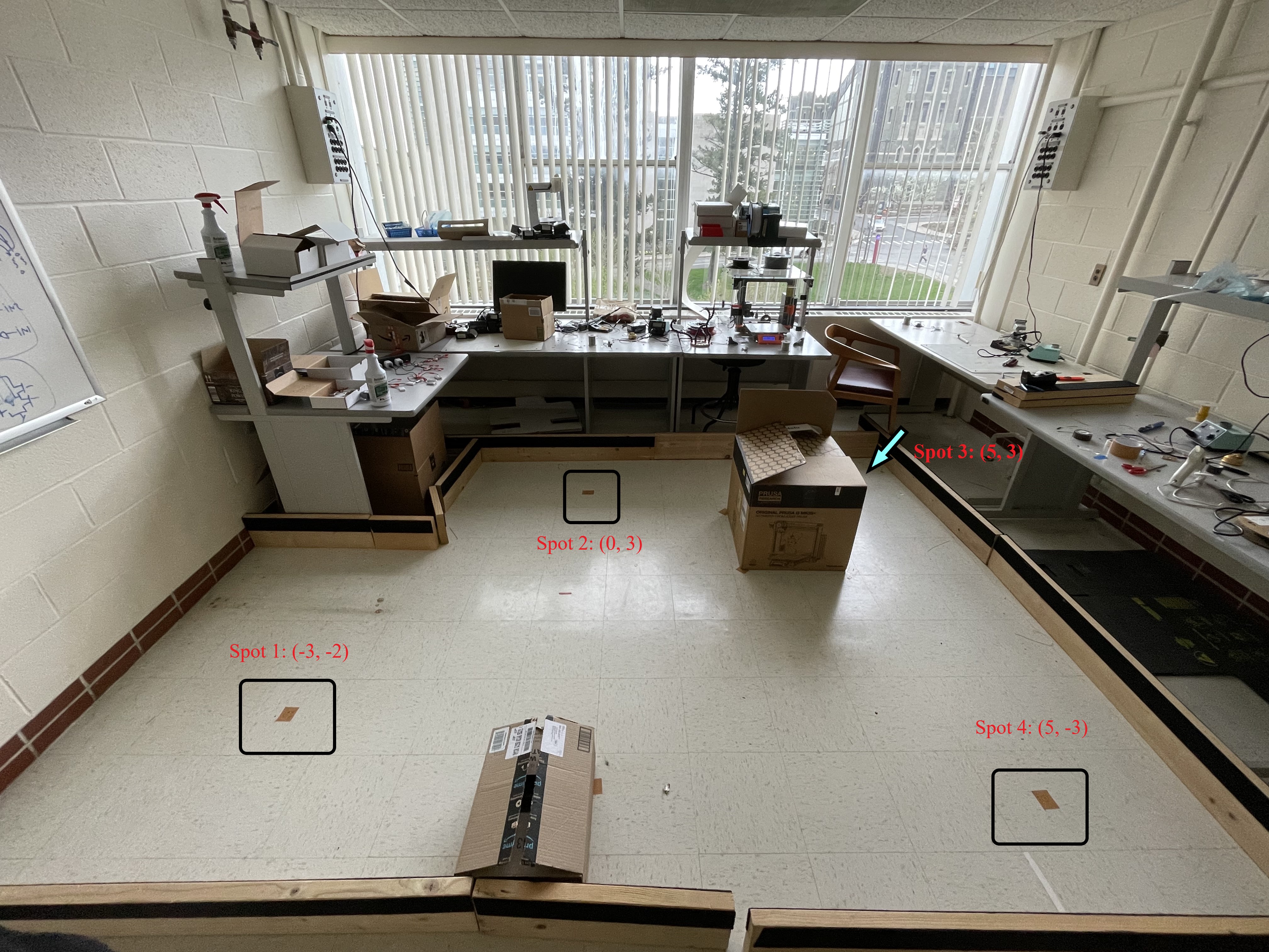The Area to Create the Map

Lab Tasks

Control: Open Loop Control

Since I am running short of time, I decide to implement open loop control to make my robot spin around on the spots to record ToF sensor readings. After conducting several tests of the spinning on a spot in the area, my open loop control program is designed as below.

Open Loop Control

I decide to collect 23 points during the 360 degree spinning, which means approximately 15.65 degrees per point, with this relatively high resolution, hopefully the point-based map can be accurate enough.

The video below shows the open loop control implemented on my robot to make it spin on the spot 3 (5, 3) collecting distance readings.

Open Loop Control

This open loop control is repeated on the five spots within the area. Below is an example plot for the implementation of open loop control on the spot 3 where the distance data is plotted in a time domain graph.

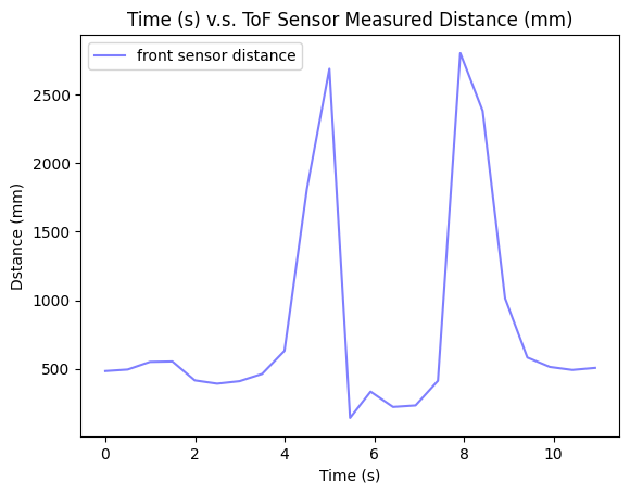Distance Data in Time Domain

The PWM duty cycle percentage during the spinning process is always 80%. My robot spins 100 ms using this PWM for approximately 15.65 degrees.

Read out Distances

To make it more intuitively to visualize the distances measured from a spot, the time domain distance plots are converted to polar plots. Since there are four marked spots within the area, I execute my turn at each of them and get the measured distances. For each spot, I conduct the turn for twice with robot placed in the same orientation to verify the precision of collected distances. It needs to be noticed that since I place my robot vertically towards the upper boundary of the area with my robot head facing forward, and my open loop control makes the robot spin clockwise, while the polar graph plots the degree increasing counter-clockwise. To fit the distance measurements with polar plot degrees properly, I conduct some transformation to change the corresponding theta angle (in radian) with respect to each distance measurement. The code snippet for the theta transformation is given as below. Eventually, the polar distance plots for the four spots are shown below, which match the real area measurement situation correctly.

Theta Transformation for Polar Plots

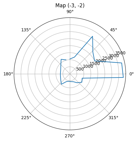Polar Plot for spot (-3, -2)

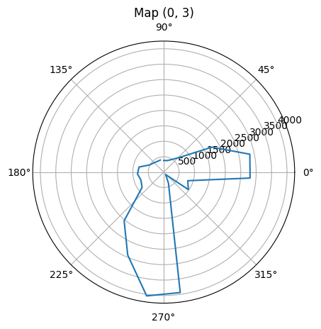Polar Plot for spot (0, 3)

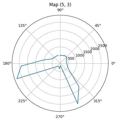Polar Plot for spot (5, 3)

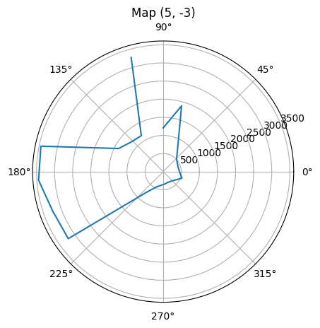Polar Plot for spot (5, -3)

Merge and Plot Readings

After I have all the measured distances for each marked spot, they are converted into x and y coordinates, and combined together to form a point-based map with different colors. Since initially, the data points in polar plots are in theta-distance format, some mathmatical operations are needed to convert them into x and y coordinates format, the code snippet for this transformation is give as:

Math Operation to Convert to X-Y Coordinate

where, theta_num is the previously transformed theta list containing radians for each distance measurements, dist_num is the distance measurements obtained from a spot, x_list and y_list are lists to store the transformed coordinates for each data point obtained by a distance measurement, and finally spot_x and spot_y are coordinates for the spot which are used to complement the distance based calculated coordinates to be equivalent to coordinates from the origin of the area. The spot_x and spot_y are actually number of tiles and are converted to mm (1 feet = 304.8 mm) when conducting coordinates transformation.

In this way, the measurements from the distance sensor are converted to the inertial reference frame of the mapping area. Since each spot has its own x and y coordinates (in feet) with respect to the center of the area. The data points are hence calibrated by adding the coordinates of the spots which the data are measured on. It needs to be notice that the unit after conversion is in mm to match the distance measurement uint (1 foot = 304.8 mm).

I write Python script to conduct the transformation process and plot the map, the code snippet is shown below.

Python Script for Data Conversion & Map Plot

Eventually, x and y coordinates of all the converted data points for each spot are plotted on the same figure with different colors as below.

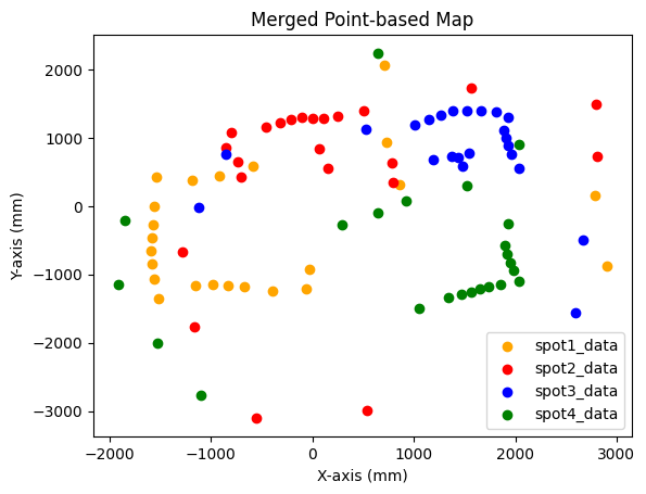Point-based Map

Line-based Map

To convert the map into a format that can be used in the simulator in future labs, the actual positions of walls and obstacles are estimated based on the scatter plotted map above. After observation, I extract some spefic "boundary" points to form lists of start and end coordinates of wall and obstacles. The points in the lists are drew in lines on top of the points-based map.

The lists of x and y coodinates for walls and boxes I extract to form the line-based map are given as below.

Lists for Line-based Map

The line-based map is hence plotted as below.

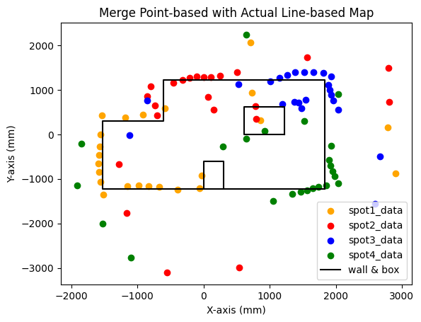Line-based Map

Texts and Videos by Zhongqi Tao